Introduction to Diffusion Models for Machine Learning

Diffusion Models are generative models which have been gaining significant popularity in the past several years, and for good reason. A handful of seminal papers released in the 2020s alone have shown the world what Diffusion models are capable of, such as beating GANs^[6] on image synthesis. Most recently, practitioners will have seen Diffusion Models used in DALL-E 2, OpenAI's image generation model released last month.

Given the recent wave of success by Diffusion Models, many Machine Learning practitioners are surely interested in their inner workings. In this article, we will examine the theoretical foundations for Diffusion Models, and then demonstrate how to generate images with a Diffusion Model in PyTorch. For a less technical, more intuitive explanation of Diffusion Models, feel free to check out our article on how physics advanced Generative AI. Let's dive in!

Diffusion Models - Introduction

Diffusion Models are generative models, meaning that they are used to generate data similar to the data on which they are trained. Fundamentally, Diffusion Models work by destroying training data through the successive addition of Gaussian noise, and then learning to recover the data by reversing this noising process. After training, we can use the Diffusion Model to generate data by simply passing randomly sampled noise through the learned denoising process.

More specifically, a Diffusion Model is a latent variable model which maps to the latent space using a fixed Markov chain. This chain gradually adds noise to the data in order to obtain the approximate posterior \( q(\textbf{x}_{1:T}|\textbf{x}_0) \), where \( \textbf{x}_1, ... , \textbf{x}_T \) are the latent variables with the same dimensionality as \( \textbf{x}_0 \). In the figure below, we see such a Markov chain manifested for image data.

Ultimately, the image is asymptotically transformed to pure Gaussian noise. The goal of training a diffusion model is to learn the reverse process - i.e. training \( p_\theta(x_{t-1}|x_t) \). By traversing backwards along this chain, we can generate new data.

Benefits of Diffusion Models

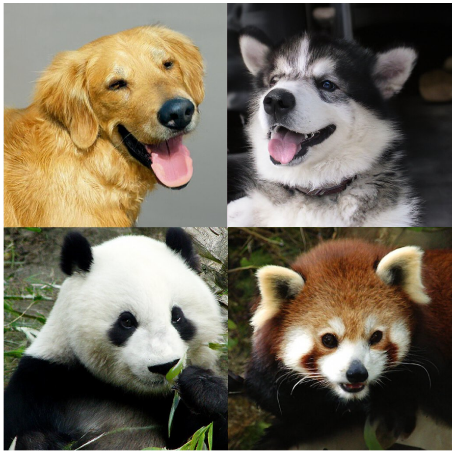
As mentioned above, research into Diffusion Models has exploded in recent years. Inspired by non-equilibrium thermodynamics^[1], Diffusion Models currently produce State-of-the-Art image quality, examples of which can be seen below:

Beyond cutting-edge image quality, Diffusion Models come with a host of other benefits, including not requiring adversarial training. The difficulties of adversarial training are well-documented; and, in cases where non-adversarial alternatives exist with comparable performance and training efficiency, it is usually best to utilize them. On the topic of training efficiency, Diffusion Models also have the added benefits of scalability and parallelizability.

While Diffusion Models almost seem to be producing results out of thin air, there are a lot of careful and interesting mathematical choices and details that provide the foundation for these results, and best practices are still evolving in the literature. Let's take a look at the mathematical theory underpinning Diffusion Models in more detail now.

Diffusion Models - A Deep Dive

As mentioned above, a Diffusion Model consists of a forward process (or diffusion process), in which a datum (generally an image) is progressively noised, and a reverse process (or reverse diffusion process), in which noise is transformed back into a sample from the target distribution.

The sampling chain transitions in the forward process can be set to conditional Gaussians when the noise level is sufficiently low. Combining this fact with the Markov assumption leads to a simple parameterization of the forward process:

Mathematical Note

We have been talking about corrupting the data by adding Gaussian noise, but it may at first be unclear where we are performing this addition. Accoring to the above equation, at each step in the chain we are simply sampling from a Gaussian distribution whose mean is the previous value (i.e. image) in the chain.

These two statements are equivalent. That is

To understand why, we will utilize a slight abuse of notation by asserting

Where the final implication stems from the mathematical equivalence between a sum of random variables and the convolution of their distributions - see this Wikipedia page for more information.

In other words, we have show that asserting the distribution of a timestep conditioned on the previous one via the mean of a Gaussian distribution is equivalent to asserting that the distribution of a given timestep is that of the previous one with the addition of Gaussian noise. We omitted the scalars introduced by the variance schedule and showed this for one dimension for simplicity, but a similar proof holds for multivariate Gaussians.

Where \( \beta_1, ..., \beta_T \) is a variance schedule (either learned or fixed) which, if well-behaved, ensures that \( x_T \) is nearly an isotropic Gaussian for sufficiently large T.

As mentioned previously, the "magic" of diffusion models comes in the reverse process. During training, the model learns to reverse this diffusion process in order to generate new data. Starting with the pure Gaussian noise \( p(\textbf{x}_{T}) := \mathcal{N}(\textbf{x}_T, \textbf{0}, \textbf{I}) \), the model learns the joint distribution \( p_\theta(\textbf{x}_{0:T}) \) as

where the time-dependent parameters of the Gaussian transitions are learned. Note in particular that the Markov formulation asserts that a given reverse diffusion transition distribution depends only on the previous timestep (or following timestep, depending on how you look at it):

Training

A Diffusion Model is trained by finding the reverse Markov transitions that maximize the likelihood of the training data. In practice, training equivalently consists of minimizing the variational upper bound on the negative log likelihood.

We seek to rewrite the \( L_{vlb} \) in terms of Kullback-Leibler (KL) Divergences. The KL Divergence is an asymmetric statistical distance measure of how much one probability distribution P differs from a reference distribution Q. We are interested in formulating \( L_{vlb} \) in terms of KL divergences because the transition distributions in our Markov chain are Gaussians, and the KL divergence between Gaussians has a closed form.

The mathematical form of the KL divergence for continuous distributions is

Below you can see the KL divergence of a varying distribution P (blue) from a reference distribution Q (red). The green curve indicates the function within the integral in the definition for the KL divergence above, and the total area under the curve represents the value of the KL divergence of P from Q at any given moment, a value which is also displayed numerically.

As mentioned previously, it is possible^[1] to rewrite \( L_{vlb} \) almost completely in terms of KL divergences:

where

Derivation Details

The variational bound is equal to

Replacing the distributions with their definitions given our Markov assumption, we get

We use log rules to transform the expression into a sum of logs, and then we pull out the first term

Using Bayes' Theorem and our Markov assumption, this expression becomes

We then split up the middle term using log rules

Isolating the second term, we see

Plugging this back into our equation for L_vlb, we have

Using log rules, we rearrange

Next, we note the following equivalence for the KL divergence for any two distributions:

Finally, applying this equivalence to the previous expression, we arrive at

Conditioning the forward process posterior on \( x_0 \) in \( L_{t-1} \) results in a tractable form that leads to all KL divergences being comparisons between Gaussians. This means that the divergences can be exactly calculated with closed-form expressions rather than with Monte Carlo estimates^[3].

Model Choices

With the mathematical foundation for our objective function established, we now need to make several choices regarding how our Diffusion Model will be implemented. For the forward process, the only choice required is defining the variance schedule, the values of which are generally increasing during the forward process.

For the reverse process, we much choose the Gaussian distribution parameterization / model architecture(s). Note the high degree of flexibility that Diffusion Models afford - the only requirement on our architecture is that its input and output have the same dimensionality.

We will explore the details of these choices in more detail below.

As noted above, regarding the forward process, we must define the variance schedule. In particular, we set them to be time-dependent constants, ignoring the fact that they can be learned. For example^[3], a linear schedule from \(\beta_1=10^{-4}\) to \(\beta_T=0.2\) might be used, or perhaps a geometric series.

Regardless of the particular values chosen, the fact that the variance schedule is fixed results in \( L_{T} \) becoming a constant with respect to our set of learnable parameters, allowing us to ignore it as far as training is concerned.

Now we discuss the choices required in defining the reverse process. Recall from above we defined the reverse Markov transitions as a Gaussian:

We must now define the functional forms of \( \pmb{\mu}_\theta \) or \( \pmb{\Sigma}_\theta \). While there are more complicated ways to parameterize \( \pmb{\Sigma}_\theta \)^[5], we simply set

That is, we assume that the multivariate Gaussian is a product of independent gaussians with identical variance, a variance value which can change with time. We set these variances to be equivalent to our forward process variance schedule.

Given this new formulation of \( \pmb{\Sigma}_\theta \), we have

which allows us to transform

to

where the first term in the difference is a linear combination of \(x_t\) and \(x_0\) that depends on the variance schedule \(\beta_t\). The exact form of this function is not relevant for our purposes, but it can be found in [3].

The significance of the above proportion is that the most straightforward parameterization of \( \mu_\theta \) simply predicts the diffusion posterior mean. Importantly, the authors of [3] actually found that training \(\mu_\theta\) to predict the noise component at any given timestep yields better results. In particular, let

where

This leads to the following alternative loss function, which the authors of [3] found to lead to more stable training and better results:

The authors of [3] also note connections of this formulation of Diffusion Models to score-matching generative models based on Langevin dynamics. Indeed, it appears that Diffusion Models and Score-Based models may be two sides of the same coin, akin to the independent and concurrent development of wave-based quantum mechanics and matrix-based quantum mechanics revealing two equivalent formulations of the same phenomena^[2].

While our simplified loss function seeks to train a model \( \pmb{\epsilon}_\theta \), we have still not yet defined the architecture of this model. Note that the only requirement for the model is that its input and output dimensionality are identical.

Given this restriction, it is perhaps unsurprising that image Diffusion Models are commonly implemented with U-Net-like architectures.

The path along the reverse process consists of many transformations under continuous conditional Gaussian distributions. At the end of the reverse process, recall that we are trying to produce an image, which is composed of integer pixel values. Therefore, we must devise a way to obtain discrete (log) likelihoods for each possible pixel value across all pixels.

The way that this is done is by setting the last transition in the reverse diffusion chain to an independent discrete decoder. To determine the likelihood of a given image \(x_0\) given \(x_1\), we first impose independence between the data dimensions:

where D is the dimensionality of the data and the superscript i indicates the extraction of one coordinate. The goal now is to determine how likely each integer value is for a given pixel given the distribution across possible values for the corresponding pixel in the slightly noised image at time \(t=1\):

where the pixel distributions for \(t=1\) are derived from the below multivariate Gaussian whose diagonal covariance matrix allows us to split the distribution into a product of univariate Gaussians, one for each dimension of the data:

We assume that the images consist of integers in \({0, 1, ..., 255}\) (as standard RGB images do) which have been scaled linearly to \([-1, 1]\). We then break down the real line into small "buckets", where, for a given scaled pixel value x, the bucket for that range is \([x-1/255, x+1/255]\). The probability of a pixel value x, given the univariate Gaussian distribution of the corresponding pixel in \(x_1\), is the area under that univariate Gaussian distribution within the bucket centered at x.

Below you can see the area for each of these buckets with their probabilities for a mean-0 Gaussian which, in this context, corresponds to a distribution with an average pixel value of \(255/2\) (half brightness). The red curve represents the distribution of a specific pixel in the t=1 image, and the areas give the probability of the corresponding pixel value in the t=0 image.

Given a t=0 pixel value for each pixel, the value of \( p_\theta(x_0 | x_1) \) is simply their product. This process is succinctly encapsulated by the following equation:

where

and

Given this equation for \( p_\theta(x_0 | x_1) \), we can calculate the final term of \(L_{vlb}\) which is not formulated as a KL Divergence:

Final Objective

As mentioned in the last section, the authors of [3] found that predicting the noise component of an image at a given timestep produced the best results. Ultimately, they use the following objective:

The training and sampling algorithms for our Diffusion Model therefore can be succinctly captured in the below figure:

Diffusion Model Theory Summary

In this section we took a detailed dive into the theory of Diffusion Models. It can be easy to get caught up in mathematical details, so we note the most important points within this section below in order to keep ourselves oriented from a birds-eye perspective:

1. Our Diffusion Model is parameterized as a Markov chain, meaning that our latent variables \(x_1, ... , x_T\) depend only on the previous (or following) timestep.
2. The transition distributions in the Markov chain are Gaussian, where the forward process requires a variance schedule, and the reverse process parameters are learned.
3. The diffusion process ensures that \(x_T\) is asymptotically distributed as an isotropic Gaussian for sufficiently large T.
4. In our case, the variance schedule was fixed, but it can be learned as well. For fixed schedules, following a geometric progression may afford better results than a linear progression. In either case, the variances are generally increasing with time in the series (i.e. \(\beta_i < \beta_j\) for \(i < j\) ).
5. Diffusion Models are highly flexible and allow for any architecture whose input and output dimensionality are the same to be used. Many implementations use U-Net-like architectures.
6. The training objective is to maximize the likelihood of the training data. This is manifested as tuning the model parameters to minimize the variational upper bound of the negative log likelihood of the data.
7. Almost all terms in the objective function can be cast as KL Divergences as a result of our Markov assumption. These values become tenable to calculate given that we are using Gaussians, therefore omitting the need to perform Monte Carlo approximation.
8. Ultimately, using a simplified training objective to train a function which predicts the noise component of a given latent variable yields the best and most stable results.
9. A discrete decoder is used to obtain log likelihoods across pixel values as the last step in the reverse diffusion process.

With this high-level overview of Diffusion Models in our minds, let's move on to see how to use a Diffusion Models in PyTorch.

Diffusion Models in PyTorch

While Diffusion Models have not yet been democratized to the same degree as other older architectures/approaches in Machine Learning, there are still implementations available for use. The easiest way to use a Diffusion Model in PyTorch is to use the denoising-diffusion-pytorch package, which implements an image diffusion model like the one discussed in this article. To install the package, simply type the following command in the terminal:

pip install denoising_diffusion_pytorch

Minimal Example

To train a model and generate images, we first import the necessary packages:

import torch
from denoising_diffusion_pytorch import Unet, GaussianDiffusion

Next, we define our network architecture, in this case a U-Net. The dim parameter specifies the number of feature maps before the first down-sampling, and the dim_mults parameter provides multiplicands for this value and successive down-samplings:

model = Unet(
    dim = 64,
    dim_mults = (1, 2, 4, 8)
)

Now that our network architecture is defined, we need to define the Diffusion Model itself. We pass in the U-Net model that we just defined along with several parameters - the size of images to generate, the number of timesteps in the diffusion process, and a choice between the L1 and L2 norms.

diffusion = GaussianDiffusion(
    model,
    image_size = 128,
    timesteps = 1000,   # number of steps
    loss_type = 'l1'    # L1 or L2
)

Now that the Diffusion Model is defined, it's time to train. We generate random data to train on, and then train the Diffusion Model in the usual fashion:

training_images = torch.randn(8, 3, 128, 128)
loss = diffusion(training_images)
loss.backward()

Once the model is trained, we can finally generate images by using the sample() method of the diffusion object. Here we generate 4 images, which are only noise given that our training data was random:

sampled_images = diffusion.sample(batch_size = 4)

Training on Custom Data

The denoising-diffusion-pytorch package also allow you to train a diffusion model on a specific dataset. Simply replace the 'path/to/your/images' string with the dataset directory path in the Trainer() object below, and change image_size to the appropriate value. After that, simply run the code to train the model, and then sample as before. Note that PyTorch must be compiled with CUDA enabled in order to use the Trainer class:

from denoising_diffusion_pytorch import Unet, GaussianDiffusion, Trainer

model = Unet(
    dim = 64,
    dim_mults = (1, 2, 4, 8)
).cuda()

diffusion = GaussianDiffusion(
    model,
    image_size = 128,
    timesteps = 1000,   # number of steps
    loss_type = 'l1'    # L1 or L2
).cuda()

trainer = Trainer(
    diffusion,
    'path/to/your/images',
    train_batch_size = 32,
    train_lr = 2e-5,
    train_num_steps = 700000,         # total training steps
    gradient_accumulate_every = 2,    # gradient accumulation steps
    ema_decay = 0.995,                # exponential moving average decay
    amp = True                        # turn on mixed precision
)

trainer.train()

Below you can see progressive denoising from multivariate Gaussian noise to MNIST digits akin to reverse diffusion:

Final Words

Diffusion Models are a conceptually simple and elegant approach to the problem of generating data. Their State-of-the-Art results combined with non-adversarial training has propelled them to great heights, and further improvements can be expected in the coming years given their nascent status. In particular, Diffusion Models have been found to be essential to the performance of cutting-edge models like DALL-E 2.

References

[1] Deep Unsupervised Learning using Nonequilibrium Thermodynamics

[2] Generative Modeling by Estimating Gradients of the Data Distribution

[3] Denoising Diffusion Probabilistic Models

[4] Improved Techniques for Training Score-Based Generative Models

[5] Improved Denoising Diffusion Probabilistic Models

[6] Diffusion Models Beat GANs on Image Synthesis

[7] GLIDE: Towards Photorealistic Image Generation and Editing with Text-Guided Diffusion Models

[8] Hierarchical Text-Conditional Image Generation with CLIP Latents